Earlier we have written blog posts about both Ohm’s Law and Kirchhoff’s Laws. It’s time to put these in action combined to analyze simple DC circuits.
Sounds fun, right!?
Don’t worry, it’s pretty easy and straight forward, and we’ll walk you through it by going through a simple example. You should read those other posts first (they’re not long) before continuing if this topic is new to you.
A Very Simple Theoretical Example
Even though we’ll continue in the theoretical domain, these examples make it much easier to understand these theoretical concepts.
The circuit below contains a 48 V voltage source, two resistors (R0 and R1) with respectively 100 Ω and 500 Ω, and a current source of 0.5 A. You can look at current sources as voltage sources which will supply a constant amount of current.
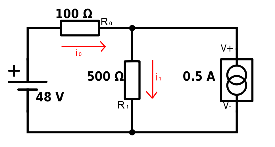
The goal in this example is to find the current values of i0 and i1. We will also automatically find out which way the current flows: if a result is positive, the current flows the same way as its corresponding arrow. And vice versa: if the result is negative, the current flows the opposite way of the arrow.
Remember that it doesn’t really matter what direction we set the arrows to point – the physical result will stay the same – but we need to define a direction for calculation purposes.
Since we have two unknowns we need to obtain two equations. We’ll use both of Kirchhoff’s two laws for this.
Applying Kirchhoff’s Current Law (KCL)
Let’s apply KCL in the top center node:
As we remember from the previous Kirchhoff blog post, KCL states that current into a node is equal to current out of the node. We have defined i1 to exit the node and i0 and the 0.5 A current from the current source to enter the node. Hence the equation above.
Applying Kirchhoff’s Voltage Law (KVL)
First, let’s find an expression for the voltage drop over the resistors. This is where Ohm’s law comes in!
This can be used to define the voltage drop over the two resistors:
Lets apply KVL in the loop to the left:

Remember that we need to have different signs on elements if they’re either sources or typical “voltage drop components” (e.g. resistors).
If we put eq. 1 into eq. 5 we get:

And with the magic of algebra, we get:
Here we have our first actual result! 0.34 A flows through R0. As we can se from the negative value, the current is actually flowing in the opposite direction of the arrow (that is from right to left) through the resistor, despite the 48 V voltage source.
From here we put the result from eq. 7 into eq. 1:

And here’s our second result. The current through R1 is 0.16 A and flows the same way as the arrow (downwards).
If you’ve had enough of equations and theory stop reading now and come back later. On the other hand, if you want to make Georg Simon and Gustav proud, man up and venture forth!
Calculating the Power Consumption and Generation
Now we’ll test the solution by verifying that the total power generated equals the total power consumed, which is an interesting exercise in itself.
Remember from pt. 1 that the equation for power is
We’ll use this to calculate power consumed/generated for each of our four circuit elements.
First, R0:

This resistor dissipates 11.56 W in the form of heat.
Then, R1:

The calculation for the voltage source is a bit different:

Since i0 is defined to go in a clockwise direction, it enters the “negative” side of the source, and the convention says that we therefore use a negative number in the equation above (-48). This is just a rule of thumb which is handy to remember.
Read more about the so called passive sign convention here!
The current (0.34 A) is negative since it goes the other way than the defined direction. The result is positive, the same as with resistors, which means that energy is consumed and not delivered to the circuit.
Lastly, we have the current source:

The voltage difference over the source is the same as over R1: 80 V. By following the same convention as with the voltage source we end up with a negative answer, which means that the source is supplying 40 W to the circuit.
Now we check if the supplied power is equal to the consumed power:

Since we have rounded some of the results and squared those several places, we don’t get an exact result, but it’s close enough.
Summary
This might not be the most relevant example out there, but the approach is applicable to many similar real-world circuits. However, remember that the fundamental principles here are much more important than the way we solved this problem.
A similar approach is also used to analyze more complex RLC circuits (circuits with resistors, inductors and capacitors). We might visit this particular topic at a later date.
The example in this post was inspired by an example from Nilson and Riedel’s Electric Circuits (8th ed., 2008).