In this blog post we’ll first briefly discuss Fourier Transform and FFT. Then we’ll show you one way to implement FFT on an Arduino.
Fast Fourier Transform (aka. FFT) is an algorithm that computes Discrete Fourier Transform (DFT). We’re not going to go much into the relatively complex mathematics around Fourier transform, but one important principle here is that any signal (even non-periodic ones) can be quite accurately reconstructed by adding sinusoidal signals together with different frequencies and amplitudes. The more sinusoidal signals we add together, the more our reconstructed signal will look like the original one. Theoretically speaking, with an infinite amount of sinusoidal signals we get an identical signal as the original.
Disclaimer: from now on we’ll only use the term FFT (for simplicity’s sake) even though DFT or just Fourier Transform might be the right term in some cases.
Below is a nice GIF which shows how six sinusoidal signals added together can resemble a square-wave signal.
FFT
The FFT-algorithm uses this principle and essentially enables you to see which frequencies are present in any analog signal and also see which of those frequencies that are the most dominating. This is very helpful in a huge amount of applications. Graphs like the blue one with only spikes (f^) in the GIF above is what you typically get after running an FFT:
- The x-axis is frequency – the higher up on this axis, the higher the frequency.
- The y-axis is amplitude – the higher up on this axis, the larger the amplitude.
What you typically get in this graph is one or more spikes. A tall spike means that that particular frequency is dominant in the signal.
If you apply FFT to a noise-free sinusoidal signal you will get only a single peak. This is logical since you only need one sinusoidal signal to recreate a sinusoidal signal.
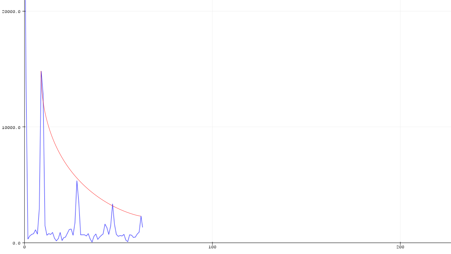
However, if you apply FFT to a square-wave signal (as shown in the GIF) you will get an exponential decreasing-looking graph, where many frequencies with an even interval between them are present. The lowest frequency have the largest amplitude (this is the primary frequency of the square-wave signal) and the highest frequencies have the lowest amplitudes.
Sampling Frequency
The Nyquist-Shannon Sampling Theorem tells us that to be able to sample a signal, the sampling frequency needs to be at least twice the frequency of the signal we’re trying to sample. In other words, the FFT will only be able to detect frequencies up to half the sampling frequency.
On a common Arduino, the sampling frequency is quite limited, though. An ADC operation (using analogRead()) takes about 100 μs, and other operations are relatively slow due to the 8 or 16 MHz clock frequency.
Number of Samples
The FFT-algorithm works with a finite number of samples. This number needs to be 2n where n is an integer (resulting in 32, 64, 128, etc). The larger this number is, the slower the algorithm will be. However, with many samples you will get a larger resolution for the results.
Bins
The term bins is related to the result of the FFT, where every element in the result array is a bin. One can say this is the “resolution” of the FFT. Every bin represent a frequency interval, just like a histogram. The number of bins you get is half the amount of samples spanning the frequency range from zero to half the sampling rate.
Arduino
There are of course several ways to implement FFT on an Arduino. You can implement it from scratch or you can use a pre-made library. In this post we’ll do the latter.
Installing the Library
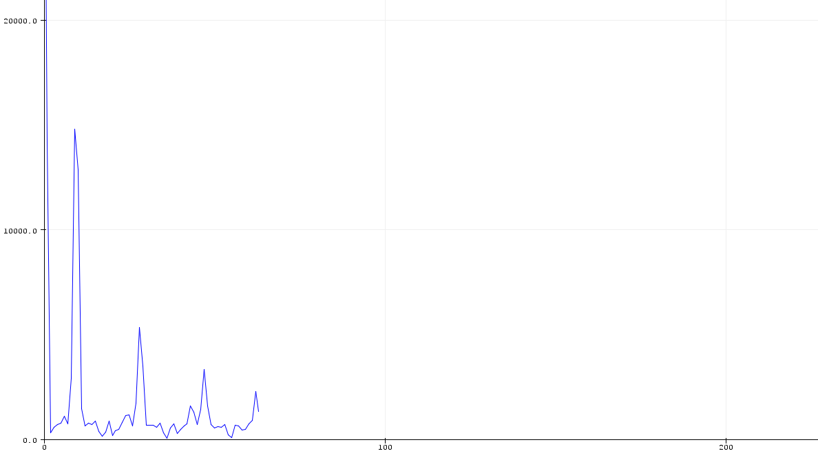
The first thing you need to do is to install the library, which is very easy. We’re using arduinoFFT by kosme, which is not to be mistaken with this library.
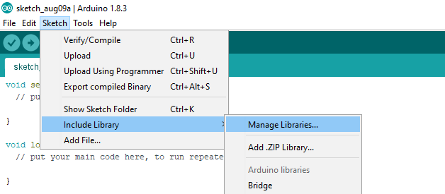
To install arduinoFFT, open the Manage Libraries window, type fft in the search bar and install the latest version.
You are now ready to start coding!
Our Example and Code
The setup we’re going to use here is an Arduino Uno and a signal generator. The only wires are the two from the signal generator where one goes to A0 on the Arduino and the other goes to GND. Our signal has an amplitude and offset such that it almost spans the complete 0-5 V range, suiting our ADC’s properties well.
Unlike the example code which comes with the library, we apply FFT to a proper analog signal. The example code generates a simulated sinusoidal signal and applies FFT to that.
Here’s the code:
#include "arduinoFFT.h"

#define SAMPLES 128 			//Must be a power of 2
#define SAMPLING_FREQUENCY 1000 //Hz, must be less than 10000 due to ADC

arduinoFFT FFT = arduinoFFT();

unsigned int sampling_period_us;
unsigned long microseconds;

double vReal[SAMPLES];
double vImag[SAMPLES];

void setup() {
	Serial.begin(115200);

	sampling_period_us = round(1000000*(1.0/SAMPLING_FREQUENCY));
}

void loop() {

	/*SAMPLING*/
	for(int i=0; i<SAMPLES; i++)
	{
		microseconds = micros();	//Overflows after around 70 minutes!

		vReal[i] = analogRead(0);
		vImag[i] = 0;

		while(micros() < (microseconds + sampling_period_us)){
		}
	}

	/*FFT*/
	FFT.Windowing(vReal, SAMPLES, FFT_WIN_TYP_HAMMING, FFT_FORWARD);
	FFT.Compute(vReal, vImag, SAMPLES, FFT_FORWARD);
	FFT.ComplexToMagnitude(vReal, vImag, SAMPLES);
	double peak = FFT.MajorPeak(vReal, SAMPLES, SAMPLING_FREQUENCY);

	/*PRINT RESULTS*/
	//Serial.println(peak);		//Print out what frequency is the most dominant.

	for(int i=0; i<(SAMPLES/2); i++)
	{
		/*View all these three lines in serial terminal to see which frequencies has which amplitudes*/

		//Serial.print((i * 1.0 * SAMPLING_FREQUENCY) / SAMPLES, 1);
		//Serial.print(" ");
		Serial.println(vReal[i], 1);	//View only this line in serial plotter to visualize the bins
	}

	//delay(1000);	//Repeat the process every second OR:
	while(1); 		//Run code once
}
This code has three “print modes”:
- Line 41 can print to terminal which frequency is most dominant.
- Lines 47-49 can print to terminal the values of each bin.
- Line 49 will print can print to plotter the visualization of all the bins.
The last two lines (52 and 53) are mutually exclusive. Either you run the FFT once or you run it repeatedly with a certain interval.
If we look towards the top of the code you can see that the number of samples is 128. The Arduino Uno does not have enough memory to support 256 samples.
You can also print the sampled signal within the sampling for-loop. Be aware that the Serial.println() function is quite slow and can impact your sampling rate.
Results
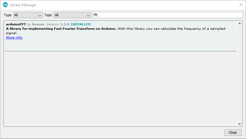
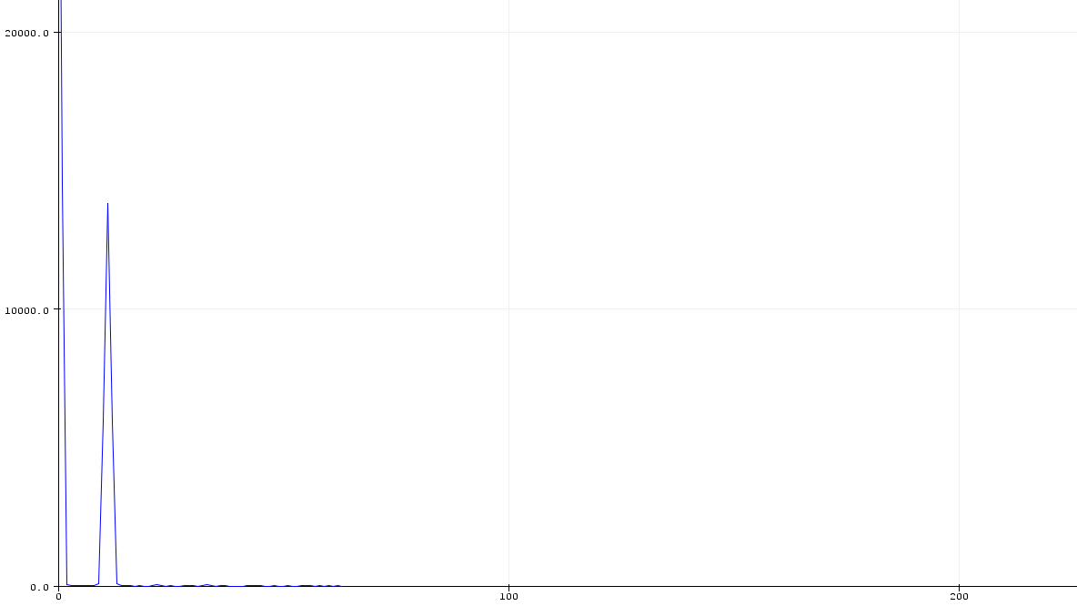
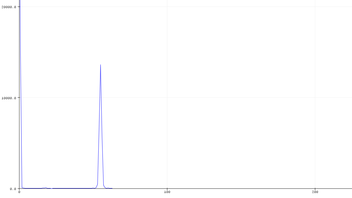
The following graphs are fetched from the Arduino serial plotter after running FFT on a few different signals with 128 Hz sampling rate and 128 samples.
The numbers on the x-axis in the graphs below are not frequency, but element number (aka. bin). In the graphs below, element number 64 is the top bin (~500 Hz). Since our input signal is has a DC offset we get the peak at zero in the results.
Last Chapter
FFT is a very handy tool in signal processing with many areas of applications. The arduinoFFT library does all the hard work for you. By using an Arduino, you’re quite limited in terms of memory and sampling rate, though. As we understand it, it’s also common to run a low-pass filter in cunjunction with the FFT algorithm, which we haven’t done in our example.
We recommend using a signal generator when starting playing with the FFT algorithm. That way you can easily change the frequency, waveforms, offset and amplitude of your signal.
Updated 12.02.18 – Peak at zero explained (thanks, Matt N)