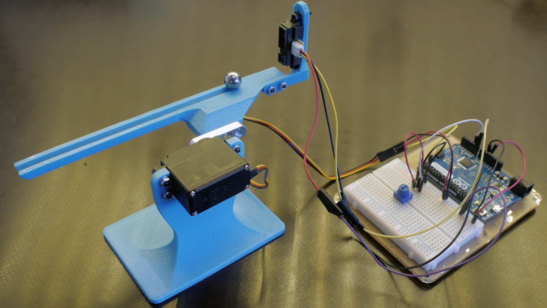
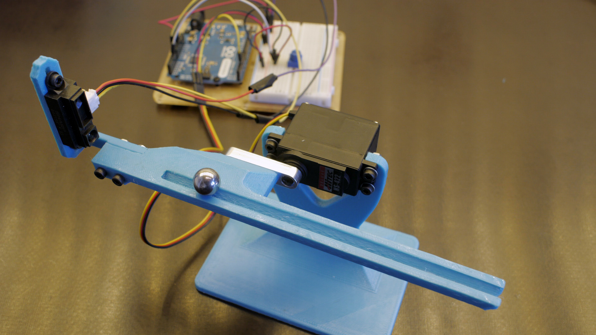
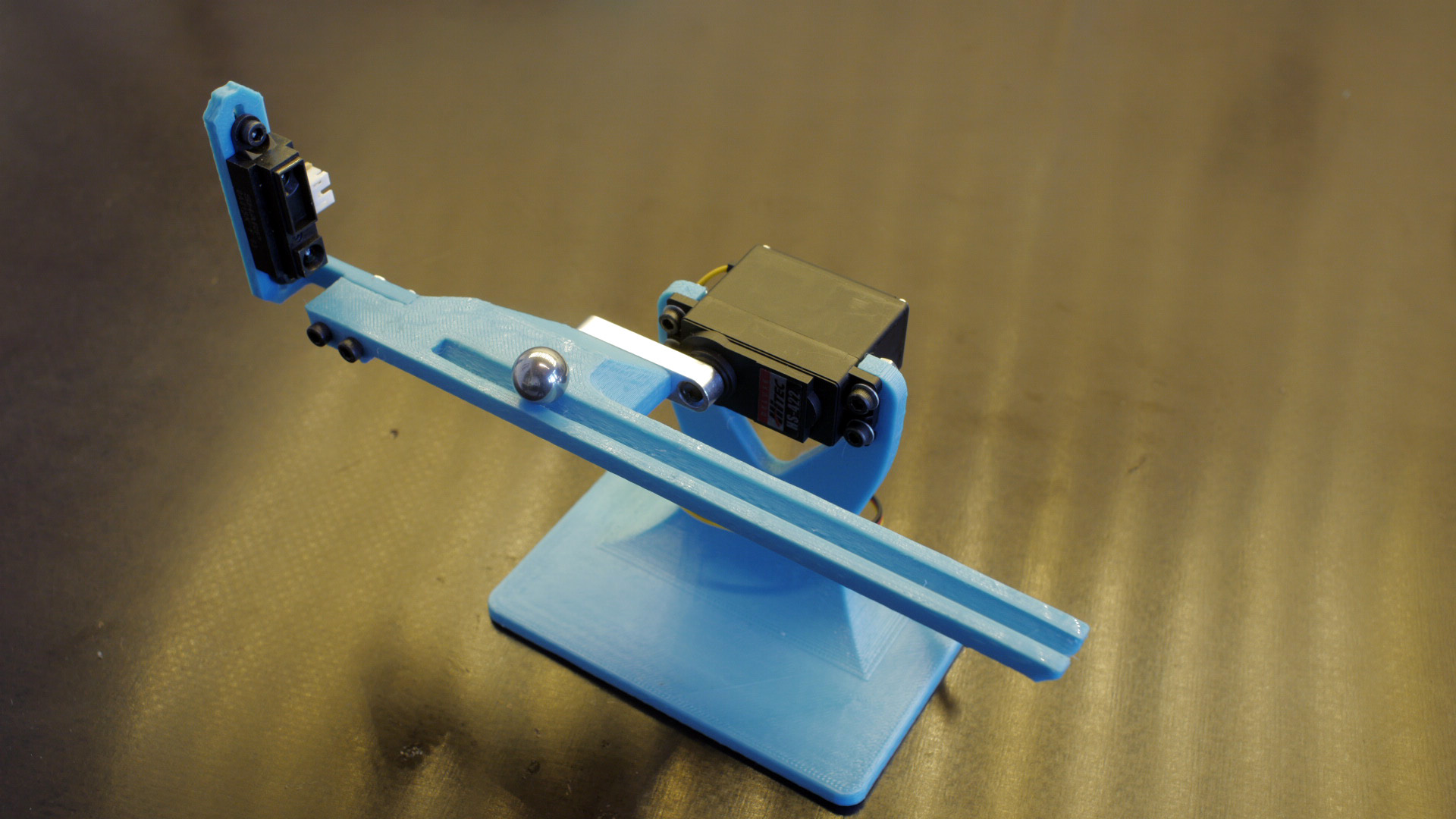
A few weeks ago we wrote a post about this small project where we’re building a seesaw which will balance a ball with the help of a proximity sensor, a servo and a PID controller implemented on an Arduino. All the parts have now arrived, the seesaw is assembled and the the firmware is implemented.
In this post we will talk about the basic theory around PID controllers, look at the implementation for this project and discuss different challenges around controlling the seesaw as well as the current performance and areas of improvement.
If you don’t care about the theory you can just go ahead and skip to the implementation part.
Basic Control and PID Theory
Controlling something physical with a computer is not as trivial as you might think. That said, when you know the basics it doesn’t have to be that complicated either.
Closed Loop Control
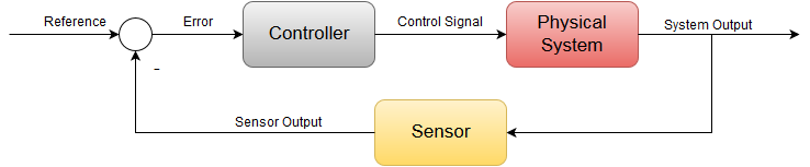
A closed loop in this case means that the controller gets feedback from the output of the system with the help of a sensor and uses that to compute a control signal which is applied to the physical system. In our case with the seesaw, the system output is the position of the ball. The reference is where we want the ball to be and the error is the difference between the reference and the system/sensor output. If the error is zero then the ball is exactly where it should be. The control signal is the signal applied to the system. In our case this is the servo position.
Stability and Damping
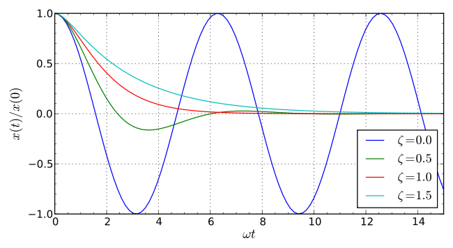
A system can be stable, unstable or marginally stable:
- A stable system will eventually converge to a steady-state.
- An unstable system will oscillate with a gradually increasing amplitude and never reach a steady-state.
- A marginally stable system will oscillate with a constant amplitude. It is the theoretic state between a stable and an unstable system.
A stable system can be overdamped, underdamped, critically damped or undamped:
- An overdamped system will reach its steady-state without oscillations (turquoise line below).
- An underdamped system will reach its steady-state after oscillating over a certain time. The amplitude will gradually decrease (green line below)
- A critically damped system system is optimally damped, i.e. it reaches the steady-state as quickly as possible without oscillating (red line below).
- An ideal undamped system without any friction may behave marginally stable (blue line below).
The PID Controller
PID control (or one of its close relatives) is probably the most common closed-loop control method. PID is an acronym for Proportional Integral Derivative, which also happens to be the three main mathematical elements (terms) of the PID controller. Depending on your system you might want to mix-and-match these terms. Some systems may only require a P, PI or a PD controller while others require the full PID package.
Each term has a coefficient which you can look at as the tuning parameters (typically named Kp, Ki and Kd). These constants decides how much each term should contribute to the overall control.
Let’s look at the three terms.
Proportional
The larger error the more gain is applied.
The P-term only takes into account the error between the sensor output and the reference. The larger error the more gain is applied (the output is proportional to the error). This might in some cases suffice as control, however you will often need something in addition to make the system stable and at the same time a bit quicker than a snail.
A large Kp results in large deviations for the control signal at large errors. This can often lead to a faster, but less dampened (or even unstable) system.
Integral
…the I-term accumulates the error over time.
This term can be related to the P-term. However, while the P term only looks at the error right now, the I-term accumulates the error over time (i.e. it intigrates the error).
This term is often added if you have problems with a steady-state error. With an I-term a small steady-state error can be accumulated to a sufficiently large error so that it is compensated for in the controller.
A large Ki will more quickly accumulate error and this can have great consequences on the stability. Integral windup is another issue. Use with care.
Derivative
You can say that while the I-term looks at the past, the D-term looks into the future.
The D-term takes the slope or the rate of change (i.e. the derivative) of the error. If the error is quickly approaching zero the D-term sees this and compensates for it. You can say that while the I-term looks at the past, the D-term looks into the future. Larger Kd results in more emphasis on the future side of things.
In an ideal world this sounds like the perfect solution for all the problems you’ll have with just the PI controller. Sadly, we’re not living in an ideal world and according to an estimate the D-term is only used in around 25% of the deployed controllers. In the real world we have noise which has a HUGE impact on the D-term. High frequencies can make it go haywire. Low-pass filtering is needed, but in some cases this might cause enough latency (time delay) from the sensor which in turn makes the system more unstable. These are tradeoffs that we will look at further down. Where you have more natural damping the negative sides with the D-term can be avoided. You also have cascaded control and many other modifications that might help.
Tuning the PID controller
An argument against using PID controllers is that it require a bit of tuning to work properly. The tuning boils down to choosing values for the coefficients Kp, Ki and Kd. There are a few “cook books” which can be utilized in some systems to make your life easier. We’re going to quickly look at one of them: the Ziegler-Nichols method.
The Ziegler-Nichols Method
The steps for using this method is in theory quite simple.
- Set Ki and Kd to zero and find which Kp (starting from zero) that results in a marginally stable system. This Kp is called Ku (ultimate gain).
- While the system is marginally stable, meassure the oscillation period Tu.
- Set Kp, Ki and Kd to values according to the table on this page.
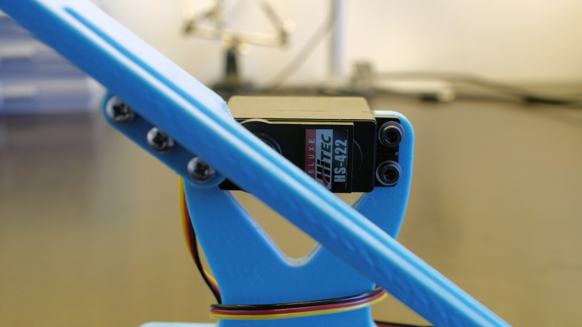
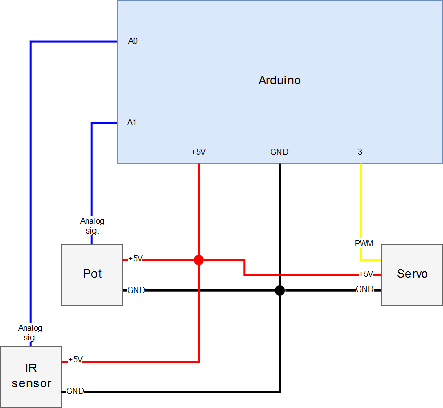
Implementing the PID Controller on the Seesaw
The implementation on a microcontroller is quite simple. Just make sure that you have a specific Δt (delta t). Δt is the time period between each time the controller is run and is used in both the I and the D-term.
For the implementation itself follow this pseudocode.
Current Performance
The seesaw is working at the moment. It balances the ball well between 4.5 and 7 cm. This is SW-range and not actual real-life range, the sensor isn’t 100% calibrated. If we bump the ball it compensates for that and returns the ball to the reference point. It also responds well to changes in the reference (via the potentiometer).
As described below the code it is struggling gradually more and more at greater ranges. It is somewhat twitchy, but within the aforementioned range it is manageable. Over time it compensates for steady-state errors as a result of the uneven gutter.
Further down we will discuss all the challenges in more detail as well as areas of improvements.
Our Code
Below is all the code we use on the Arduino.
#include <Servo.h>

/*SERVO POSITION CONSTANTS*/
#define SERVO_OFFSET 1425   //center position
#define SERVO_MIN 1000
#define SERVO_MAX 1900

/*REFERENCE RANGE*/
#define REFERENCE_MIN 4.5
#define REFERENCE_MAX 7.0

/*DELTA T*/
#define DT 0.001  //seconds

/*PID PARAMETERS*/
#define Kp 0.7    //proportional coefficient
#define Ki 0.2    //integral coefficient
#define Kd 0.2    //derivative coefficient

/*UPSCALING TO Servo.writeMilliseconds*/
#define OUTPUT_UPSCALE_FACTOR 10

/*EMA ALPHAS*/
#define SENSOR_EMA_a 0.05
#define SETPOINT_EMA_a 0.01

/*SENSOR SPIKE NOISE HANDLING*/
#define SENSOR_NOISE_SPIKE_THRESHOLD 15
#define SENSOR_NOISE_LP_THRESHOLD 300

float mapfloat(float x, float in_min, float in_max, float out_min, float out_max);

Servo myservo;

/*ARDUINO PINS*/
int sensor_pin = 0;
int pot_pin = 1;
int servo_pin = 3;

/*EMA VARIABLE INITIALIZATIONS*/
float sensor_filtered = 0.0;
int pot_filtered = 0;

/*GLOBAL SENSOR SPIKE NOISE HANDLING VARIABLES*/
int last_sensor_value = analogRead(sensor_pin);
int old_sensor_value = analogRead(sensor_pin);

/*GLOBAL PID VARIABLES*/
float previous_error = 0;
float integral = 0;

void setup() {
  Serial.begin(115200);
  myservo.attach(servo_pin);
}

void loop() {
  /*START DELTA T TIMING*/
  unsigned long my_time = millis();

  /*READ POT AND RUN POT EMA*/
  int pot_value = analogRead(pot_pin);
  pot_filtered = (SETPOINT_EMA_a*pot_value) + ((1-SETPOINT_EMA_a)*pot_filtered);

  /*MAP POT POSITION TO CM SETPOINT RANGE*/
  float setpoint = mapfloat((float)pot_filtered, 0.0, 1024.0, REFERENCE_MIN, REFERENCE_MAX);

  /*READ SENSOR DATA*/
  int sensor_value = analogRead(sensor_pin);

  /*REMOVE SENSOR NOISE SPIKES*/
  if(abs(sensor_value-old_sensor_value) > SENSOR_NOISE_LP_THRESHOLD || sensor_value-last_sensor_value < SENSOR_NOISE_SPIKE_THRESHOLD){  //everything is in order
	old_sensor_value = last_sensor_value;
	last_sensor_value = sensor_value;
  }
  else{                               //spike detected - set sample equal to last
	sensor_value = last_sensor_value;
  }

  /*LINEARIZE SENSOR OUTPUT TO CENTIMETERS*/
  sensor_value = max(1,sensor_value);         //avoid dividing by zero
  float cm = (2598.42/sensor_value) - 0.42;

  /*RUN SENSOR EMA*/
  sensor_filtered = (SENSOR_EMA_a*cm) + ((1-SENSOR_EMA_a)*sensor_filtered);

  /*PID CONTROLLER*/
  float error = setpoint - sensor_filtered;
  integral = integral + error*DT;
  float derivative = (error - previous_error)/DT;
  float output = (Kp*error + Ki*integral + Kd*derivative)*OUTPUT_UPSCALE_FACTOR;
  previous_error = error;

  /*PRINT TO SERIAL THE TERM CONTRIBUTIONS*/
  //Serial.print(Kp*error);
  //Serial.print(' ');
  //Serial.print(Ki*integral);
  //Serial.print(' ');
  //Serial.println(Kd*derivative);

  /*PRINT TO SERIAL FILTERED VS UNFILTERED SENSOR DATA*/
  //Serial.print(sensor_filtered);
  //Serial.print(' ');
  //Serial.println(cm);

  /*PREPARE AND WRITE SERVO OUTPUT*/
  int servo_output = round(output) + SERVO_OFFSET;

  if(servo_output < SERVO_MIN){ //saturate servo output at min/max range servo_output = SERVO_MIN; } else if(servo_output > SERVO_MAX){
	servo_output = SERVO_MAX;
  }

  myservo.writeMicroseconds(servo_output);  //write to servo

  /*PRINT TO SERIAL SETPOINT VS POSITION*/
  //Serial.print(sensor_filtered);
  //Serial.print(' ');
  //Serial.println(setpoint);

  /*WAIT FOR DELTA T*/
  //Serial.println(millis() - my_time);
  while(millis() - my_time < DT*1000);
}

float mapfloat(float x, float in_min, float in_max, float out_min, float out_max)
{
 return (x - in_min) * (out_max - out_min) / (in_max - in_min) + out_min;
}
Real-world Challenges
Controlling a system in theory is so much easier than in real life. Here are some of the challenges we faced in this project.
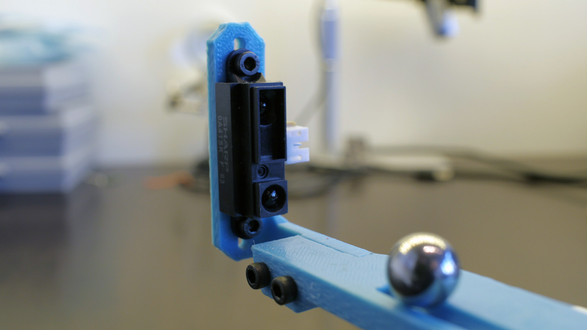
Sensor Noise
The proximity sensor is a noisy motherf****r, especially when the ball is further away from the sensor. It probably picks up signals from the gutter itself and the surroundings. After all, the ball gets smaller and smaller the further away from the sensor it rolls. The sensor also behaves differently between having a wall in the background and just air.
We’re running an Exponential Moving Average (EMA) filter on the sensor data. Here we quickly get into a tradeoff fight: too much noise or too slow readings – a classic lesser evil situation.
A periodic cluster of spikes is also part of the noise. These spikes are handled before the EMA by comparing the current sample with the previous one. If the difference is above a certain threshold the sample is discarded. We also have a low-pass threshold which looks at the difference between the current sample and an even older sample. If the difference is above a different larger threshold no samples are discarded since we actually have a large change in readings and not noise spikes.
Despite these noise countermeasures we still get a heavy impact on the PID controller’s D-term, making it pretty twitchy.
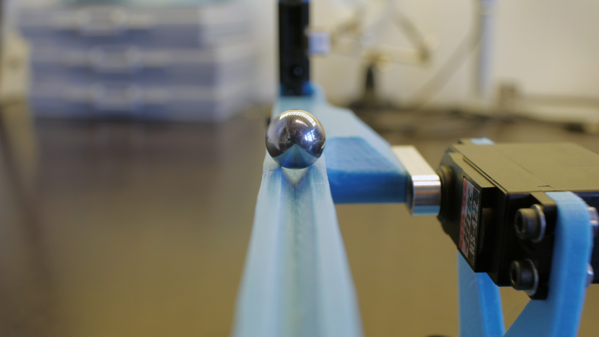
Uneven Gutter
The 3D-print is not super slick. It has a few small bumps which makes the ball stay a bit more in place at some spots. This often results in a steady-state error, and therefore we need the I-term to compensate for this.
Servo Resolution
We started using the Servo.write() function, but we quickly saw that it was too coarse resolution-wise. Servo.writeMilliseconds() works better. We kept the PID tuning parameters and just upscaled the controller output. This resulted in a bit better performance.
Δt
The control process has to be done at certain time-intervals. That is, they can’t be done continuously. We started with a Δt of 5 ms, but after looking at how little time the control loop used, even with printouts over serial (less than 1 ms) we set Δt to 1 ms and it seemed to improve the performance somewhat.
Tuning the PID Controller
We gave the Ziegler-Nichols method a shot, but didn’t get further than step 1. We were not able to find a Kp which resulted in a remotely stable system. In physical systems like this you’ll often find it extremely difficult to apply the Ziegler-Nichols method, especially when you have such low natural damping as we have here. Filtering latency, somewhat uneven gutter and poor servo resolution does not help either. So from there on out is was trial and error.
We set Kp to where it behaved sensibly and wasn’t too much aggressive. A larger Kp makes it unstable.
Due to the small bumps in the gutter we needed an I-term (steady-state errors are not cool). To avoid integral windup Ki had to be pretty small.
Kd proved to be the real pain in the ass. We needed the D-term to achieve stability while at the same time it was the reason for a very twitchy servo behaviour due to the sensor noise. We tweaked it to a (not so) golden mean, but we acheived acceptable behaviour.
Room for Improvements
The seesaw is by no means perfect. Here are some areas that can be improved:
Reposition the Rotational Axis
If the servo rotational axis is positioned at the center of the gutter instead of the center of the whole construction we would mitigate some of the vertical bumpyness applied to the ball on the far end of the gutter. We must then sacrifice the symmetric min/max servo limit for all you OCD people out there, but the servo never travels that far anyway.
Better Noise Filtering
EMA doesn’t seem to work great in this application. It gets too slow too soon. Without having done too much research in the area there should exist better forms for low-pass filtering. Maybe a combination of HW and SW filtering would work as well. The spike reduction could also probably do with some refinement.
Smoother Gutter
The gutter got a bit bumpy since we had to remove a brim used to stick the print properly to the 3D-printer bed. This would probably have gone better if we tried again. An alternative is to use a 3D-printer service such as Shapeways. A different option is to laser cut acrylic to get a smooth edge.
A Better Sensor Solution
This is probably the biggest issue as it stands now. The sensor struggles when the ball rolls further away than 10 cm. It is noisy and fairly unpredictable. A capacitive meassurement along the gutter would’ve been ideal.
Another solution could be to use two identical sensors, one on each end of the gutter. The two sensors could then meassure one half of the gutter each. The useful range would then be extended, but the noise would still persist. If we didn’t want an extended gutter range we could use two sensors to better filter the signal instead.
Better Servo (Control)
We don’t think that the servo necessarily needs to be faster. However, an even better resolution would probably be somewhat benefitial.
Different Controller
You have alternative control methods such as LQR, MPC and Kalman filtering. These are more complex control methods than your everyday PID controller. Whether these are worth implementing, or even applicable to our system, is not certain at this time. If we’ll ever find out remains to be seen.